Josselin has attended:
Excel Advanced course
Excel VBA Intro Intermediate course
Formatting with 5 conditions
Good afternoon,
I am trying to format the background of cells depending on their values.
To simplify, I'd like to change the background colour of the cell to:
- Dark blue if the value of the cell is less than 100
- Light blue if the value of the cell is between 100 and 0.
- Green is the value is between 0 and 100.
- Orange of the value is between 100 and 200.
- Red if the value is greater than 200.
Although I understand how I would do it with an "IF" function, I am having some problem with the conditional formatting. I have also thought about do it with VBA but would prefer start with Excel conditional formatting first.
In reality, I am looking for a VLOOKUP value in a different page as set value and also would need to apply an "AND" function to make sure this VLOOKUP value is enabled (marked with a "T"), such that a true statement would be:
IF(AND(VLOOKUP("Tag",limits,13)="T", A4>VLOOKUP("Tag",limits,12))) then change the background colour in red.
limits being the table where I take the VLOOKUP value from.
Which is also giving me some errors...
Can you please give me some guidance and the best way to replicate this conditional formatting to 100s of cells.
Thank you,
J
RE: Formatting with 5 conditions
Hi Joss
Good to hear from you again. I want to clarify a few points before we talk about a solution.
Your conditional formatting rules: the first three conditions overlap. e.g. if I use the value "50" it meets the criteria for dark blue, light blue and green. Have some of your figures not come out right? It is possible to do this successive colouring, using IF logic, in the Conditional Formatting window, but we need to make sure of those boundary figures first.
With regards to your nested VLOOKUP / IF you can't encourage a function to change formatting option. You could return a value which you then use for the basis of your conditional formatting. What error are you seeing?
Kind regards
Gary Fenn
Microsoft Office Specialist Trainer
Tel: 0207 987 3777
Best STL - https://www.stl-training.co.uk
98%+ recommend us
London's leader with UK wide delivery in Microsoft Office training and management training to global brands, FTSE 100, SME's and the public sector
RE: Formatting with 5 conditions
Thanks for you quick response Gary.
Indeed, I forgot "-" in from of my 2 first conditions.
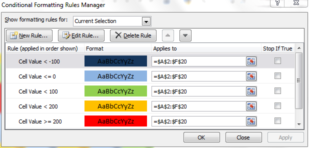
- Dark blue if the value of the cell is less than -100
- Light blue if the value of the cell is between -100 and 0.
- Green is the value is between 0 and 100.
- Orange of the value is between 100 and 200.
- Red if the value is greater than 200.
As for the second part of the question, I think I am going to put it on hold for now and work around the Excel conditional formatting first.
Regards,
Joss
RE: Formatting with 5 conditions
Hi Joss
That makes sense! Yes, structure it like a nested IF function, working your way through the boundaries from lowest to highest.
I've attached a workbook where I've employed this (select the data and go to Conditional Formatting > Manage Rules) and a screenshot of the ruleset.
In each case I've added a new rule and chose "Format only cells that contain", setting the criteria and formatting style each time. Note every time you add a rule you can use the up / down arrows to move the rule up or down in order of precedence.
Kind regards
Gary Fenn
Microsoft Office Specialist Trainer
Tel: 0207 987 3777
Best STL - https://www.stl-training.co.uk
98%+ recommend us
London's leader with UK wide delivery in Microsoft Office training and management training to global brands, FTSE 100, SME's and the public sector


