Conditional Formatting for dates to be highlighted after years.

Hi

Thanks for getting in touch. With this Conditional Formatting you need to use a formula to calculate it correctly.

The TODAY() function will work out today's date. If you subtract 21 days (3 x 7) you know what the date is 3 weeks before today.

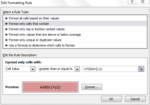
Highlight your dates and go to Conditional Formatting > New Rule > Format Only Cells that contain...

Change the drop-down from "between" to "greater than or equal to" and in the formula type =TODAY()-21

Then under Format choose your style (red fill etc).

This should then highlight any date greater than ("after") today's date 3 weeks ago.

I hope that helps, I've included a screenshot of the rules window to help you out. Here's a useful link describing more of these conditional formatting tricks in detail:

http://www.techonthenet.com/excel/questions/cond_format4_2010.php

Kind regards

Gary Fenn
Microsoft Office Specialist Trainer

Tel: 0207 987 3777
Best STL - https://www.stl-training.co.uk
98%+ recommend us

London's leader with UK wide delivery in Microsoft Office training and management training to global brands, FTSE 100, SME's and the public sector

Hi Joyce

Thank you for your question

As I understand it the conditional format should be based on a formula that compares the training due date in the cell with today's date. If today's date is within 3 weeks for the due date the the conditional format should trigger and highlight the due date.

Click on the first date to be formatted
on the Home tab choose conditional formatting
From the menu choose new rule
set the rule to be based on a formula

the formula could look like this (replace A1 with the selected cell reference, make sure you remove any dollars that Excel may add)

=(A1-TODAY())<=21

This formula works out the difference between the due date and today's date. If the difference is less than or equal to 21 days then the conditional highlight will trigger.

You can use the format painter paintbrush to copy and apply the conditional format to the rest of the sheet.

Let me know if this produces the result you are looking for. As always test first on a backup copy to make sure it meets your requirements before using it for real.

Kind regards,
Andrew

File has been uploaded from delegate

Hi Joyce

Thanks for the file. I've made a change to the Conditional Formatting in the range B5:B16. I've emailed this to you.

Please note, to test it out I also added two dates that weren't in the original list in B13 and B14. One is more than 3 weeks away, and one is definitely within 3 weeks.

I hope this helps.

Kind regards

Gary Fenn
Microsoft Office Specialist Trainer

Tel: 0207 987 3777
Best STL - https://www.stl-training.co.uk
98%+ recommend us

London's leader with UK wide delivery in Microsoft Office training and management training to global brands, FTSE 100, SME's and the public sector