Lisa has attended:
Excel Introduction course
Excel Intermediate course
Excel Advanced course
Conditional Formatting for Highlighting Dates
Hi,
Can you please advise how I can get a date cell to change colour (be highlighted) to indicate an upcoming end date within say, the next calendar month? But not for dates beyond that?
Thanks,
Lisa
RE: Conditional Formatting for Highlighting Dates
Hi Lisa
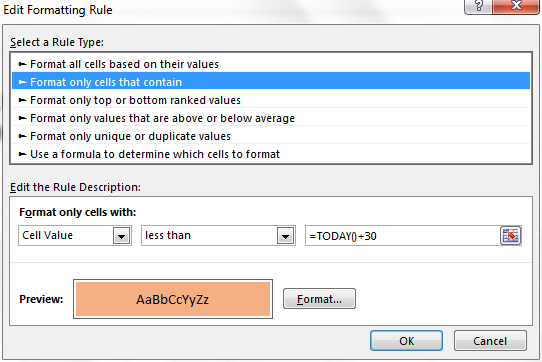
Thanks for getting in touch. You'll need to use a specific type of Conditional Formatting to achieve this. The following rule will highlight any date that is less than (before) today's date plus thirty days.
Select your date cells, then on the Home tab go to Conditional Formatting > New Rule.
Choose Format only cells that contain:
Cell Value | Less than | =TODAY()+30
Then press Format and choose your formatting style. I've attached an image of what the window should look like when you're finished.
Kind regards
Gary Fenn
Microsoft Office Specialist Trainer
Tel: 0207 987 3777
Best STL - https://www.stl-training.co.uk
98%+ recommend us
London's leader with UK wide delivery in Microsoft Office training and management training to global brands, FTSE 100, SME's and the public sector
Attached files...
RE: Conditional Formatting for Highlighting Dates
Hi Gary,
That worked really well. Off the back of that just a couple of other things... :-)
I already have some conditional formatting in place which seems to have been overwritten by the new conditioning, can you not have multiple conditioning rules on cells?
Also, how might I get the above to turn a whole row into a colour if the condition is met within that one cell and not just the cell?
Thanks,
Sorry can of worms!
RE: Conditional Formatting for Highlighting Dates
Hi Lisa
Thanks for your reply. All possible, with differing degrees of difficulty!
For your first question, you can have theoretically unlimited rules on a single cell / selection. Your latest rule is coming last and overriding the others. To edit this, select the affected cells, go to Home > Conditional Formatting > Manage rules. Your rules will be listed here. Click the up / down arrows to move the rules up and down in order of execution, and pay attention to the Stop if true option, will will halt any further conditional formatting rules being applies.
For the second question, you can do it but you'll have to be a bit more precise in your rules. The method I listed earlier will _not_ work for this. Select all the cells to be affected by the rule and go back to New rule and select Use a formula to determine which cells to format.
Assuming your first date is in cell A1, try the following formula:
=$A1<TODAY()+30
Then choose your formatting as before. The dollar signs in that reference are *very* important. Do change your column / row to the first occurrence of the date in your table.
Give it a go and let me know how you get on.
Kind regards
Gary Fenn
Microsoft Office Specialist Trainer
Tel: 0207 987 3777
Best STL - https://www.stl-training.co.uk
98%+ recommend us
London's leader with UK wide delivery in Microsoft Office training and management training to global brands, FTSE 100, SME's and the public sector


