Conditional Formatting is one of the most powerful tools in Excel. It can do so much to help you track data with relatively little time and effort. This ‘Quick Win’ tool can be mastered in a few simple steps. The blog will look at what Conditional Formatting is, how to apply it to data and what it can be useful for to improve performance tracking.

What is Conditional Formatting
Conditional Formatting is based on setting rules or conditions on specific data and if any of this data meets a rule then it will change its appearance in some way e.g. display an icon or change colour (see below)

In this example there are 3 separate rules all set according to specific bands or ranges of numbers. If a number falls into a specific band, then it will change to the appropriate colour. The world of finance has coined the term ‘RAG’ status – or Red, Amber, Green – to represent low, medium and high numbers. Excel has many pre-set icons and colour ranges to help you adopt this useful tracking system.
Why use Conditional Formatting
Think of situations where you might find this technique useful. For example, someone in HR might need to track all staff whose monthly sick days are greater than 4. Or an Events Organiser might want to colour code for each client on their books. Maybe an administrator needs to show when deadlines are about to be hit within 2 days, hit already or deadline has already passed all in different colours. Whatever the scenario, Conditional Formatting can vastly improve your data analysis techniques thus making you more productive.
How to apply Conditional Formatting
- Open ‘Revenue Table’ or similar dataset in Excel.
- Highlight all the sales figures and go to HOME > CONDITIONAL FORMATTING > HIGHLIGHT CELLS RULES:

- Select BETWEEN from the sub-list. This action brings up the following dialog box with red already set to a specific band:
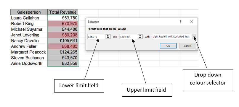
- To customise your own bands, start with the highest first. Enter 100000 (lower limit) and 150000 (upper limit). From the ‘Drop down colour selector’, choose ‘Green Fill with Dark Green text’:

- With the figures still highlighted, repeat steps 2-4 setting the following rules/colours:

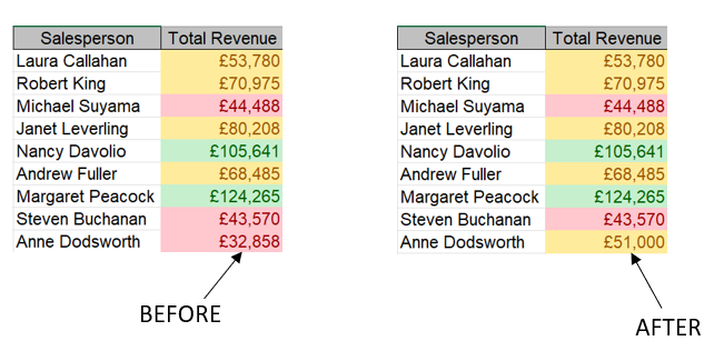
- The really amazing feature of Conditional Formatting once it’s created is that it is dynamic, i.e. the data will change colour if it meets the corresponding rule.
- For example, Ann Dodsworth’s revenue has increased to £51,000 so her revenue figure has changed from red to yellow (or amber):
Conclusion
Conditional Formatting in Excel can really help you understand your data in order to make insightful business decisions which in turn leads to greater profitability.