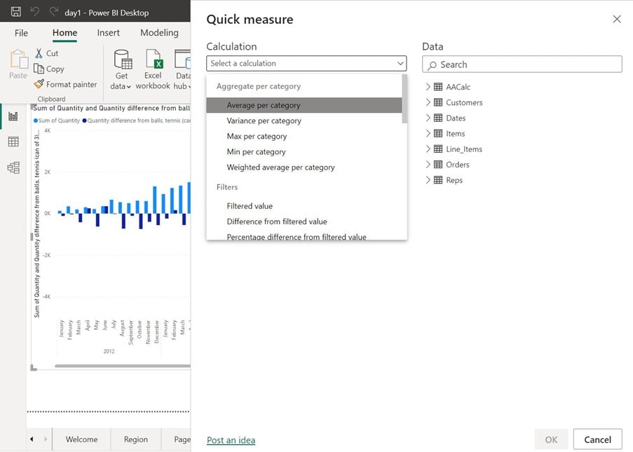
Microsoft has prepared Power BI to make it easier for users to perform DAX measures without a lot of DAX knowledge.
To access the Quick Measures, click QUICK MEASURES on the Home tab. You will see a list of options to choose from. On the right side of the Quick Measure dialog box, you will find all the tables from your data model.
Example 1 – Rolling Average
Many use rolling average to smoothing the data set. Unusual periods can be disrupting for understanding patterns and especially in projections, they can make forecasts unnecessarily inaccurate.
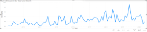
In the example below a line chart visualises sales numbers over several years, but a number of periods were unusual and you want the audience to understand how the quantity would look under normal conditions.

From the dialog box you can select the Quick Measure ‘Rolling Average’ from the Calculation list. You will now need to add the fields from your tables and set up the parameters.
In this example the quantity is the Base value, Dates are added to the Date field (Rolling Average is a Time Intelligent measure and the primary key from the timetable needs to be added), and Periods before and after are set to 3 months (the smoothing level).

When you click OK Power BI will the write the DAX.
Quantity rolling average =
IF(
ISFILTERED(‘Dates'[Dates]),
ERROR(“Time intelligence quick measures can only be grouped or filtered by the Power BI-provided date hierarchy or primary date column.”),
VAR __LAST_DATE = ENDOFMONTH(‘Dates'[Dates].[Date])
VAR __DATE_PERIOD =
DATESBETWEEN(
‘Dates'[Dates].[Date],
STARTOFMONTH(DATEADD(__LAST_DATE, -3, MONTH)),
ENDOFMONTH(DATEADD(__LAST_DATE, 3, MONTH))
)
RETURN
AVERAGEX(
CALCULATETABLE(
SUMMARIZE(
VALUES(‘Dates’),
‘Dates'[Dates].[Year],
‘Dates'[Dates].[QuarterNo],
‘Dates'[Dates].[Quarter],
‘Dates'[Dates].[MonthNo],
‘Dates'[Dates].[Month]
),
__DATE_PERIOD
),
CALCULATE(SUM(‘Line_Items'[Quantity]), ALL(‘Dates'[Dates].[Day]))
)
)
By adding the Rolling Average to the line chart, you can see the result below.

Example 2 – Percentage difference from filtered value.
The line chart below (the columns) shows sales in 3 different countries Canada, Mexico, and United States. It shows how much is generated in sales by Canada and Mexico by percentage.
The line is calculated by another Quick Measure – Percentage difference from filtered value.

In this example the Base Value is a sales measure. You can define how you want this quick measure the handle blanks. You can display them as blanks or you can tell the measure to treat blanks as zero. In this example the measure is filtered by country, and we have selected United States.

And as in the first example Power BI will write the DAX.
sales % difference from U.S.A. =
VAR __BASELINE_VALUE = CALCULATE([sales], ‘Customers'[Country] IN { “U.S.A.” })
VAR __MEASURE_VALUE = [sales]
RETURN
IF(
NOT ISBLANK(__MEASURE_VALUE),
DIVIDE(__MEASURE_VALUE – __BASELINE_VALUE, __BASELINE_VALUE)
)
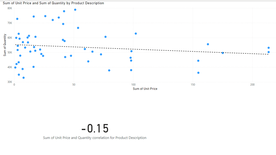
Example 3 – Correlation Coefficient
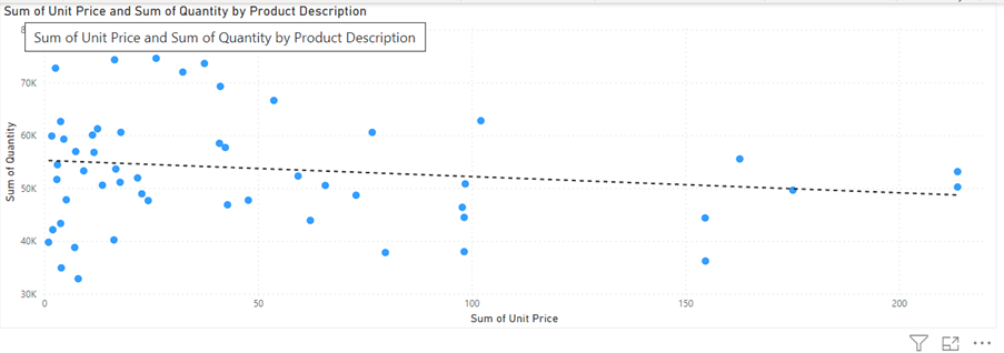
In this example correlation between product unit prices and sales quantity needs to be investigated. Does the price affect the quantity sold?
The quantity and unit price have been added to a scatter chard below. The trend line will indicate to us the relationship between the two. The dots are spread out. This indicates that there isn’t a close relationship between the two variables, but what is the correlation coefficient?
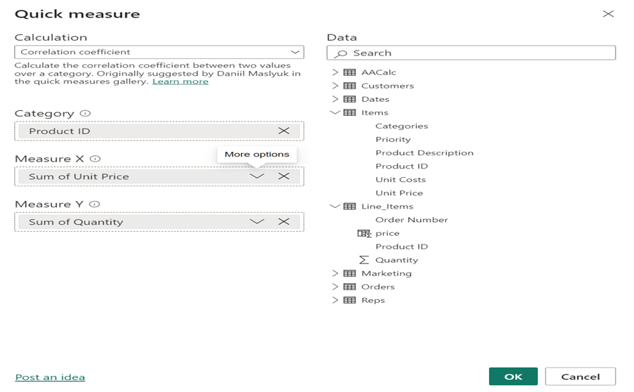
A Quick Measure can very simply find the result.
Category here is the products identified by the field Product ID. Measure X and Measure Y are the here the sum of quantity and sum of unit price.
Again, Power BI will write the DAX.
Sum of Unit Price and Quantity correlation for Product ID =
VAR __CORRELATION_TABLE = VALUES(‘Items'[Product ID])
VAR __COUNT =
COUNTX(
KEEPFILTERS(__CORRELATION_TABLE),
CALCULATE(SUM(‘Items'[Unit Price]) * SUM(‘Line_Items'[Quantity]))
)
VAR __SUM_X =
SUMX(
KEEPFILTERS(__CORRELATION_TABLE),
CALCULATE(SUM(‘Items'[Unit Price]))
)
VAR __SUM_Y =
SUMX(
KEEPFILTERS(__CORRELATION_TABLE),
CALCULATE(SUM(‘Line_Items'[Quantity]))
)
VAR __SUM_XY =
SUMX(
KEEPFILTERS(__CORRELATION_TABLE),
CALCULATE(SUM(‘Items'[Unit Price]) * SUM(‘Line_Items'[Quantity]) * 1.)
)
VAR __SUM_X2 =
SUMX(
KEEPFILTERS(__CORRELATION_TABLE),
CALCULATE(SUM(‘Items'[Unit Price]) ^ 2)
)
VAR __SUM_Y2 =
SUMX(
KEEPFILTERS(__CORRELATION_TABLE),
CALCULATE(SUM(‘Line_Items'[Quantity]) ^ 2)
)
RETURN
DIVIDE(
__COUNT * __SUM_XY – __SUM_X * __SUM_Y * 1.,
SQRT(
(__COUNT * __SUM_X2 – __SUM_X ^ 2)
* (__COUNT * __SUM_Y2 – __SUM_Y ^ 2)
)
)
The correlation between unit price and quantity here is -0.15. In other words when a product gets more expensive the sold quantity decreases. But a negative correlation of -0.15 isn’t much. Nevertheless it could be a clever idea to keep an eye on this number over time to understand the sales pattern.
Conclusion
Microsoft has given their clients a shortcut to create DAX measures by offer the quick measure tool. Quite complicated measures can be achieved without prior DAX knowledge.