How to ‘Freeze Panes’ in Excel

How often when using Excel have you had to scroll down to find what you’re looking for in a huge spreadsheet only to find your top headings disappear off the screen? Well worry no more. The solution lies in using an incredibly handy tool called Freeze Panes. This tool ‘freezes’ the top row and left column headings making it easier to check data against the appropriate headings when scrolling. This can increase your productivity and save you so much time

What are Freeze Panes

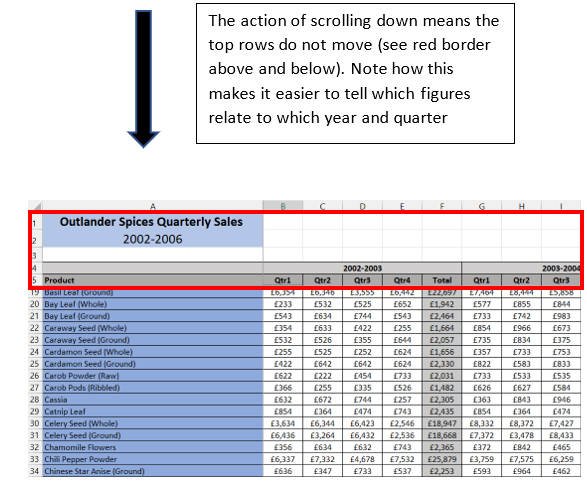
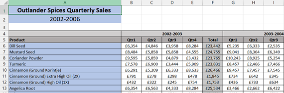
The images below show 2 separate ways to ‘freeze’ panes:

1. Freezing top rows, scroll down

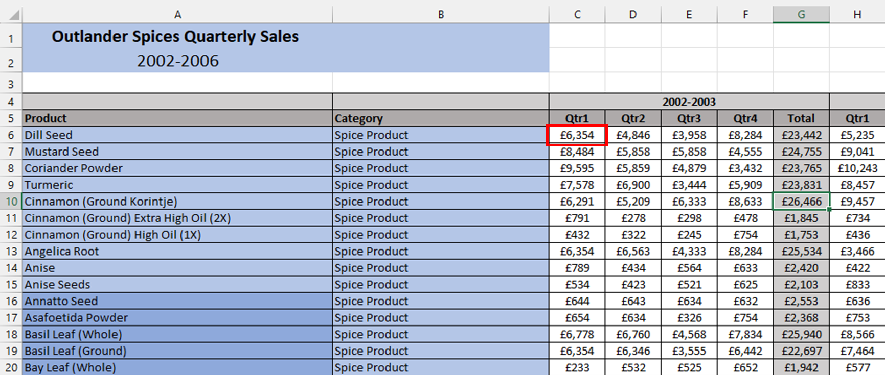
2. Freezing left columns, scroll right

 

When freezing panes there are 3 options:

1. Freeze top row (i.e. row 1)
2. Freeze first column (i.e. column A)
3. Freeze both rows and columns

The first 2 options can only be applied separately whilst the 3^rd option applies the ‘freezing’ in both directions.

How to apply Freeze Panes

 

1. To apply Freeze Panes to the top row (row 1) go to VIEW > FREEZE PANES > FREEZE TOP ROW
2. For the first column, go to VIEW > FREEZE PANES > FREEZE FIRST COLUMN

3. To ‘freeze’ both rows and columns select the cell B6 (in this example). This means when you go to VIEW > FREEZE PANES > FREEZE PANES, any rows above and to the left of cell B6 will be ‘frozen’ when scrolling in either direction

4. After ‘Freeze Panes’ has been applied, you may wish to turn off this feature. This may be because you might want to reset the areas to be frozen or you just want to take it back to normal. To do this, go to VIEW > FREEZE PANES > UNFREEZE PANES
5. If you add more columns and/or rows to your spreadsheet, you will need to ‘refreeze’ the panes. For example, adding 1 column to the left would mean selecting cell C6 and then going to VIEW > FREEZE PANES > FREEZE PANES

Conclusion

‘Freeze Panes’ is a great time saving tool that will help you organise data in large worksheets and will therefore make you more efficient in viewing your data.