
In Excel 365 and Excel 2021 Microsoft has provided Excel users with some new features which will fundamentally change the way worksheets are designed. Dynamic array formulas allow you to work with multiple values at the same time in a formula.
Dynamic arrays solve some challenging difficulties in Excel and will be a feature which will make Excel users capable of building more streamlined Excel models which more effectively can help decision makers.
Dynamic arrays are resizable arrays that calculate automatically and return values into multiple cells based on a formula entered in a single cell.
Dynamic arrays are a new feature in Excel that allows you to work with arrays of data more efficiently and will reduce time spend on updating/changing analysis and Excel reports.
Dynamic array formulas return a set of values into neighbouring cells, also known as an array. This behaviour is called spilling.
Microsoft expands the list of dynamic array formulas frequently but when this blogpost was written the list included the formulas:
ARRAYTOTEXT, BYCOL, BYROW, CHOOSECOLS, CHOOSEROWS, DROP, EXPAND, FILTER, HSTACK, ISOMITTED, LAMBDA, LET, MAKEARRAY, MAP, RANDARRAY, REDUCE, SCAN, SEQUENCE, SORT, SORTBY, STOCKHISTORY, TAKE, TEXTAFTER, TEXTBEFORE, TEXTSPLIT, TOCOL, TOROW, UNIQUE, VALUETOTEXT, VSTACK, WRAPCOLS, WRAPROWS, XLOOKUP, and XMATCH.
Example 1 – SEQUENCE
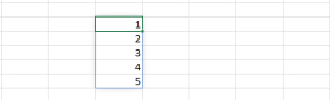
The SEQUENCE function allows you to generate a list of sequential numbers in an array, such as 1, 2, 3, 4.
=SEQUENCE (rows, [columns], [start], [step])
=SEQUENCE(5) will return this array:
 =SEQUENCE(5,5) will return this array:
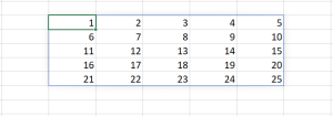
Start number and incremental steps can be entered as function arguments but in the above examples only number of rows and columns have been entered in the function.
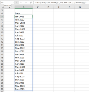
Task: Build a dynamic Excel list which always shows expenses for the last two years starting from last day previous month and two years backward.
If the following is typed in the first cell (done 31/1/2024)
=TEXT(DATE(YEAR(TODAY())-2,SEQUENCE(24,1),1),”mmm-yyyy”)
It will result in:
To make this example easier to understand will it be broken down in a couple of steps:
DATE(YEAR(TODAY())-2,SEQUENCE(24,1),1)
The DATE functions arguments are DATE(YEAR,MONTH,DAY).
In the DATE function’s year argument, the year has been extracted from the TODAY() (current date) minus 2 to go two years backward.
In the DATE function’s month argument, the SEQUENCE function has been told to generate and array with 24 rows and 1 column. In the DATE function’s day argument is just entered 1 to start from the first of the month.
=TEXT(DATE(YEAR(TODAY())-2,SEQUENCE(24,1),1),”mmm-yyyy”)
A TEXT function has been put around to tell Excel to return the date format “mmm-yyyy”.
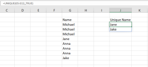
Example 2 – UNIQUE
The UNIQUE function returns a list of unique values in a list or range.
=UNIQUE (array, [by_col], [exactly_once])
=UNIQUE(G5:G12) will return this array:
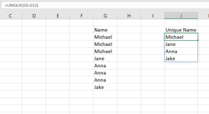
=UNIQUE(G5:G12,,TRUE) will return this array (only distinct names):
Example 3 – Best practice designing a worksheet for data analysis by using dynamic array formulas.
Dynamic array formulas can make you able to design Excel worksheets which are fully automated and self-cleaning. No more time spend when the next month data are available. No need to delete old data. No need to update calculations or formulas to include newly added data. The dynamic array formulas can take you to a completely new level of efficiency as an Excel user.
Task: Build a dynamic Excel list which always shows advertising stats, number of sales calls, and sales figures for the last three years starting from last day previous month and three years backward.
This company generates a list with monthly advertising expenses and number of sales calls their sales team has done. The sales records are broken down on day, product, and sales reps.
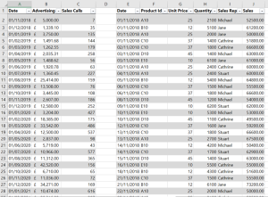
The Excel analysis should provide the company with information about the correlation between sales and advertising expenses and sales calls.
In this example 3 dynamic array formulas are used.
The TAKE function returns a specified number of contiguous rows or columns from the start or end of an array.
=TAKE(array, rows,[columns])
The SORT function sorts the contents of a range or array.
=SORT(array,[sort_index],[sort_order],[by_col])
The SORTBY function sorts the contents of a range or array based on the values in a corresponding range or array.
=SORTBY(array,by_array,[sort_order],[array/order],…)
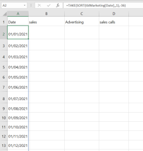
Step 1 – get the data from the source to the worksheet.
Both source lists are in tables. The list with advertising and sales calls is in a table named tblMarketing and the sales records in a table named tblSales.
To get the last 36-month dates from the tblMarketing table the TAKE function has been used.
=TAKE(tblMarketing[Date],-36)
The TAKE function has been told to create an array from the last 36 entries from the source table’s date column.
To make sure that it is always the dates from the last 36 month a SORT function has been nested inside the TAKE function.
SORT(tblMarketing[Date],,1)
The last argument in the SORT function is 1 to sort ascending.
All together the functions look like this:
=TAKE(SORT(tblMarketing[Date],,1),-36)
Step 2 is to get the advertising and sales calls from the source to the destination list.
=TAKE(tblMarketing[[Advertising]:[Sales Calls]],-36,2)
Here the TAKE function has both columns in the array argument tblMarketing[[Advertising]:[Sales Calls]] and the last argument 2 tells the TAKE function to return a two column array and again the last 36 rows.
To take sure to get the last 36 month a SORTBY function is nested. The two columns need to be sorted by the Date column.
=TAKE(SORTBY(tblMarketing[[Advertising]:[Sales Calls]],tblMarketing[Date],1),-36,2)
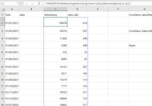
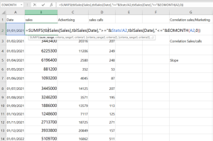
To be able to calculate the correlation the sales numbers also need to be brought in. Here is a SUMIFS function used.
Summary
Dynamic Arrays are a huge change to Excel formulas and maybe the biggest change ever. This is a game changer for all Excel users from industries such as finance, healthcare, and retail, well from all industries. As discovered through Excel London training, this can dramatically reduce time heavy tasks and make Excel users much more efficient. This blog post just scratches the surface of how this impact the way we can work with dynamic arrays in Excel.