 If you’ve got a lot of data, it’s not always easy to spot trends and to easily analyse your figures. Conditional Formatting can instantly show you patterns in your data by highlighting cells that meet certain conditions. So for example you might want to flag up sales below a certain threshold in red, or bold occurrences of a certain word. This feature has been present in Excel for years, but in Excel 2013 there’s a faster way to get to visualise patterns.
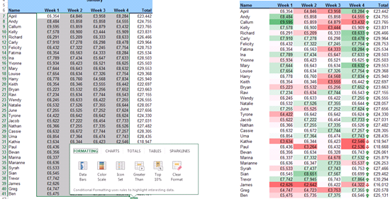
Excel 2013 has introduced Formatting through Quick Analysis. In the below example, Colour Scale Formatting is used to look for high and low spots and highlighting them as such.
How to: Highlight some Excel data in a table and look for the Quick Analysis tag to float over the bottom-right corner of your selection. Put your mouse over this icon to explore the options.
Icon Set is another option available under Quick Analysis formatting. For example totals meeting a target display a green arrow or a red arrow if they don’t.
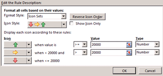
Suggested options not doing it for you? You can always create your own Conditional Formatting rules.
How to: Conditional Formatting > Manage Rules (to define the target criteria)
For more tips and features on Excel 2013 and other versions, browse Excel courses online from Best STL, available London and UK wide.