VLOOKUP is one of the most useful and versatile functions in Excel. As you work further with macros it’s not uncommon to make your create an Excel VBA VLOOKUP macro. With this you get the ability to reference your tables of data, but automated.
Wait, what’s a VLOOKUP function?
The Vertical Lookup is one of Excel’s most popular commands. It’s most common use allows you retrieve data from another table of data based on a key value. For example, in one Excel sheet you may have a list of one customer’s invoice numbers, and in another sheet a list of all your invoice numbers plus other columns, such as amount, customer and invoice date. A VLOOKUP function can use the invoice number as a reference point to extract one or more other related columns of data. This avoids sloppy copy-and-paste and ensures the data remains up to date.
There are other smart uses of the VLOOKUP, such as being able to search for duplicates, group values into buckets and check to see if items exists but this is enough detail for now.
So what about using Excel VBA VLOOKUPs?
You can retrieve data from sheet to sheet programmatically using VBA alone, usually with nested FOR NEXT loops and variables to track your current cell position. These can be a bit fiddly and the learning curve can be a little steep.
Luckily, VBA provides you with the Application.WorksheetFunction method which allows you to implement any Excel function from within your macro code.
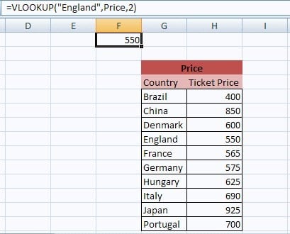
So if your original VLOOKUP in cell B2 was something like this:
=VLOOKUP(Input!A2, Data!A1:X200, 5, FALSE)
The VBA version would look like this:
Range("B2") = Application.WorksheetFunction.VLookup(Sheets("Input").Range("A2"), Sheets("Data").Range("A1:X200"), 5, False)
Notice a couple of things: I had to insert the Sheets and Range objects so VBA could properly interpret it.
I want a sneakier version!
Don’t want to do that Sheets and Ranges business? You can adopt a little-known punctuation trick in VBA that converts things into cell references: the square brackets. Did you know you can turn this:
Range("A1") = "Fred"
into
[A1] = "Fred"
With a little lateral thinking we can do the same to our VLOOKUP:
[B2] = [VLOOKUP(Input!A2, Data!A1:X200, 5, FALSE)]
Make it more robust
The code lines above will do the bare minimum. They’ll get the job done. What if you grab the result of the VLOOKUP and store it in a variable?
result = [VLOOKUP(Input!A2, Data!A1:X200, 5, FALSE)]
And then throw an unexpected value at it?
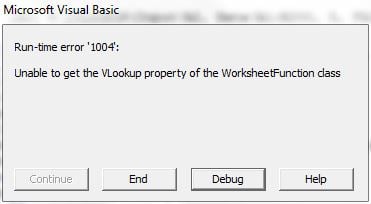
Let’s add a little error-handling so your code doesn’t come to a screeching halt. There’s a number of ways you can test this, and various things you can do with the error, so here’s only one suggestion:
On Error GoTo MyErrorHandler:

  result = [VLOOKUP(Input!A2, Data!A1:X200, 5, FALSE)]

MyErrorHandler:
  If Err.Number = 1004 Then
    MsgBox "Value not found"
  End If
Or possibly
On Error GoTo MyErrorHandler:

  result = [VLOOKUP(Input!A2, Data!A1:X200, 5, FALSE)]

MyErrorHandler:
  If Err.Number = 1004 Then
    result = ""
  End If
The first example throws the error right up in your face. The second one is a ‘silent’ error that pushes a null string into the result variable. Not usually advisable as you can’t actually spot the problem but on some occasions you just want to move past the code issue. You could replace the empty string with your own custom error message.
Make it dynamic
This is all well and good but what if your data grows and shrinks? You should be on the lookout for dynamic methods. You can consider things such as dynamic range names and similar, but here’s a VBA option you can consider:
    Dim ws As Worksheet
    Dim LastRow As Long
    Dim TargetRange As Range

    On Error GoTo MyErrorHandler:

    Set ws = Sheets("Data")

    LastRow = ws.Cells(Rows.Count, "X").End(xlUp).Row
    Set TargetRange = ws.Range("A1:X" & LastRow)

    result = Application.WorksheetFunction.VLookup(Sheets("Input").Range("A2"), TargetRange, 5, False)

    MsgBox result

MyErrorHandler:
    If Err.Number = 1004 Then
      MsgBox "Value not found"
    End If
Note I went back to standard sheet and range references; they’re tricky to mix and match with square bracket notation.
What’s happening here? We set up three variables, to house the sheet name, last row and final range. Then we calculate what the last used row is with the “xlUp” method. This is equivalent to pressing CTRL + up on the keyboard when working in Excel. This finds the last row on the worksheet, and finally we set this as the range used.
There’s lots of variations on this, depending on whether you need dynamic columns too and how regular your data is, but this is a great method for getting you started.
So there it is, from soup to nuts, ways to implement VLOOKUP functions in Excel VBA.
Looking for help on your VBA projects? We offer the UK’s largest schedule of advanced Excel courses London, with all versions and levels trained. The Introduction and Intermediate levels will give you all the tools you need to get started, while the Advanced course will allow you to hook up other Office applications and communicate with databases. We can also visit your offices to deliver training, or consult on your projects. We can also offer Access VBA and Word VBA too.