Excel 2013: 3 New Ways To Customise Your Charts

new feature for microsoft office 2013Whether you’ve decided to use a suggested chart to represent your data or already knew which one works best from the outset, a new toolbar in Excel 2013 allow you to customise your visualisation quicker.

Selecting the chart will automatically reveal two tool ribbons: Design & Format, both specifically designed to help you manipulate your Excel 2013 charts. Although the Chart Tools Layout tab no longer exists in 2013, the buttons it contained are still available, just in different places.

Excel 2013 charts

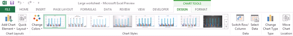
Three (new) buttons for chart formatting now appear at the top right corner of your chart; Chart Elements, Chart Styles and Chart Filters. Instead of digging through menus you can access these buttons overlaid on the chart.
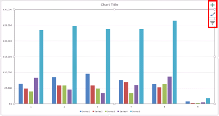
Excel 2013 charts


Chart Elements

Add or Remove specific elements of your chart such as Data Labels and Gridlines. This way you can have as much or as little labelling and layout features as you desire.
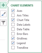
Excel Charts 2013


Chart Styles

Change the colour and style of your chart with this simple formatting option. Scroll over each option to get a preview of how your new chart will look.
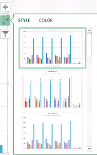
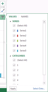
Excel Charts 2013


Chart Filters

Want to modify what data the chart includes? Previously you had to modify the data range in a fiddly way. Now you can hide and show data with the chart filters selecting them from the tick box menu, very similar to filtering data in a table. Customising your charts has never been so easy.

Excel Charts 2013


For more tips and features on Excel 2013 and other versions, browse London Excel courses from STL, available London and UK wide. With training levels ranging from beginner up to advanced and Excel VBA, there’s sure to be a course to suit your needs.

Excel : Audit your Spreadsheet with the Inquire Add-In

new feature for microsoft office 2013For users with the Office Professional Plus package, the Inquire add-in comes pre-installed on Excel 2013. Helping you to analyse, audit and review workbooks, this great new feature also has the potential to highlight errors and security concerns.

We recently discussed, how to take back control of your spreadsheets by reducing “fat finger mistakes” and auditing errors, which can have huge cost implications to businesses. The Inquire add-in is another great tool for preventing these issues from arising and escalating in Excel.

The new tool can be accessed via the Inquire Tab in the ribbon and includes a number of useful functions:

Worksheet relationship

  1. Workbook analysis
  2. Workbook relationship
  3. Worksheet relationship
  4. Cell relationship
  5. Compare files
  6. Clean Excess Cell formatting
  7. Workbook passwords

These seven functions are simple to use, many providing visualisations to help better understand the information.

We all know Excel for being data driven, however, visualising things often makes this mass data easier to understand, take for example recommended charts & graphs or all new quick analysis techniques.

A few of our favourite Inquire features include:

Cell Relationship in Excel 2013

  • Cleaning excess formatting, including formatting in blank cells which bloats file size and contributes to poor performance in Excel.
  • The ability to compare two workbooks, highlighting cells that differ. This is particularly useful during an audit.
  • Being able to visualise the relationships between cells. Understanding the audit trail of how a figure came to be is a great way of maintaining the integrity and accuracy of the data.

How to: Enable the Add-in through File > Options > Add-Ins, from the Manage drop-down choose COM Add-Ins > Go. Tick Inquire and click OK.

To use it select the Inquire Tab in Ribbon > Choose function

For more tips and features on Excel 2013 and other versions, browse Microsoft training Excel courses from STL, available London and UK wide.