Quickly create drop down lists in Excel with automatic sorting
The Drop Down list in Excel is a great automation tool. You can turn any data list into a drop down list which makes it easier to place items in cells. Drop down lists show the data in the same order in which they appear in the original list.
This may be a problem if you want your drop down list to be in alphabetical order while your original data should not be sorted. If the drop down list is long, it will take forever to find items if they are not sorted. Also, many data sets are dynamic (new records are added all the time). In this case, you need to keep altering the list range in your Data Validation which manages the list.
In this tutorial, you will learn how to create drop down lists which expand dynamically and sort alphabetically by default.
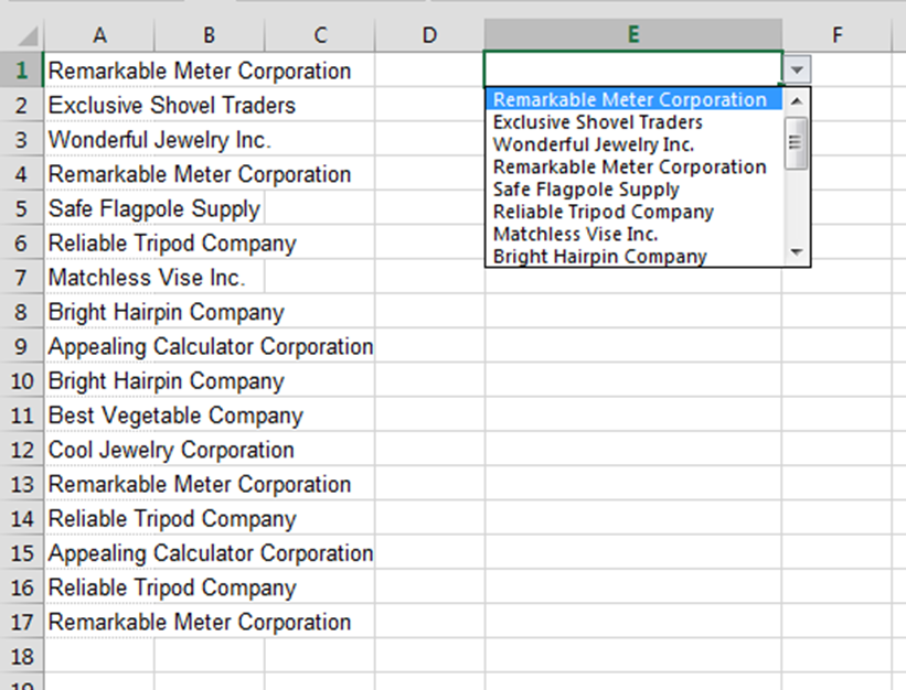
A normal drop down list looks like this:
To make the data list and the drop down dynamic as well as making the drop down alphabetical, follow these steps:
Step 1. Select the original list and give it a dynamic range name (which automatically includes new entries). See below.
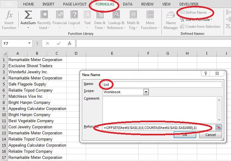
Example of formula in ‘Refers to’ field:
=OFFSET(Sheet1!$A$1, 0, 0, COUNTA(Sheet1!$A$1:$A$1000))
When you type the Offset formula into the ‘Refers to’ field, make sure the cell references reflect the position and size of your list, e.g. $A$1:$A$2000 if you have 1000+ records. You can make this any number of rows.
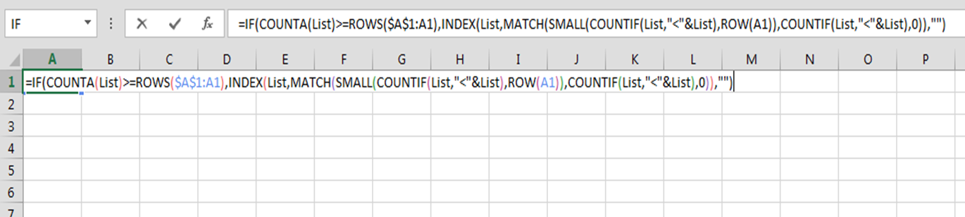
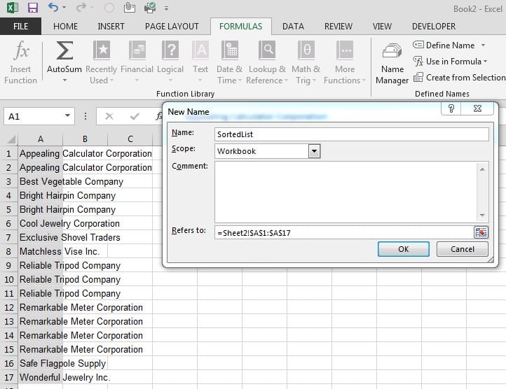
Step 2. The next step is to open a new or existing empty sheet where you can enter a formula which will create a copy of the original list, but sorted alphabetically. You must enter the formula manually and then press Ctrl + Shift + Enter to make it work. if you only press Enter, it will give an error. Here is an example of the formula:
=IF(COUNTA(List)>=ROWS($A$1:A1), INDEX(List, MATCH(SMALL(COUNTIF(List, “<“&List), ROW(A1)), COUNTIF(List, “<“&List), 0)), “”)
‘List’ in the formula represents the range name you gave your original list earlier.
Once you have typed the formula and pressed Ctrl + Shift + Enter, copy this formula down until it shows an empty cell. This means all the records of the original list are in this list.
After copying this formula down, your alphabetised list will show. Next, highlight this list and give it a range name.
The last step is to create the drop down list using the range name as the source.
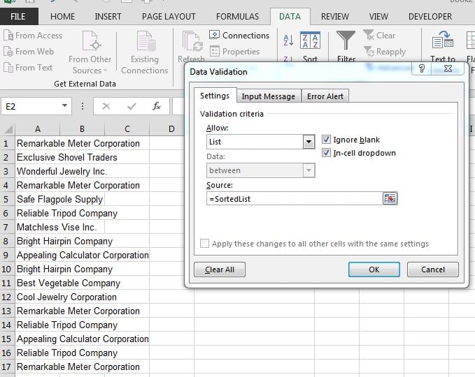
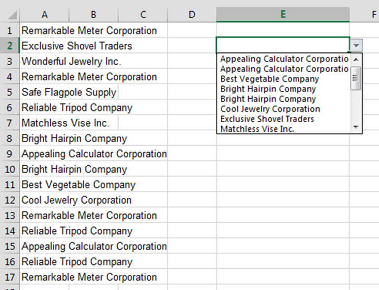
You have just created a drop down list which will dynamically update with the original list, and which will always be in alphabetical order!