The IPMT function allows you to work out the Interest payment based on the set criteria as outlined in the syntax below.
Syntax
IPMT(rate,per,nper,pv,fv,type)
Rate is the interest rate per period.
Per is the period for which you want to find the interest and must be in the range 1 to nper.
Nper is the total number of payment periods in an annuity.
Pv is the present value, or the lump-sum amount that a series of future payments is worth right now.
Fv is the future value, or a cash balance you want to attain after the last payment is made. If fv is omitted, it is assumed to be 0 (the future value of a loan, for example, is 0).
Type is the number 0 or 1 and indicates when payments are due. If type is omitted, it is assumed to be 0.
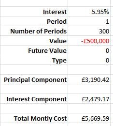
The first thing you might want to do is set up your spread sheet and format accordingly. This is an example of how I would set up my spreadsheet and what it will end up looking like. Please note on my example I have used both the PPMT and the IPMT functions. I have added a short blog on the PPMT function on this site.
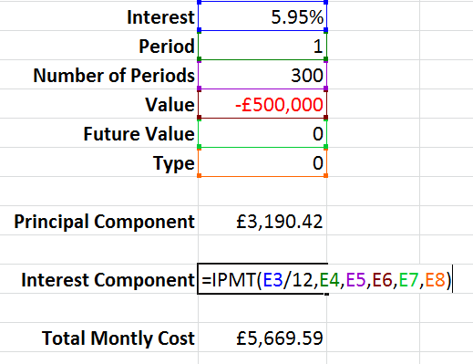
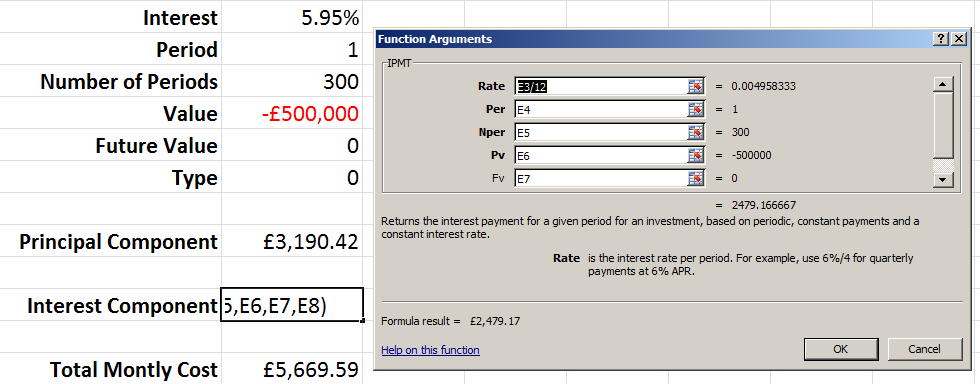
In the cell to the right of the INTEREST COMPONENT where you see “£2,479.17” is where you will enter your IPMT function. This is what it will look like if you use your INSERT FUNCTION option;
You will notice that way I have suggested you set up your spread sheet mirrors the options shown in this box and that makes entering the correct information a pretty simple process. Two things you need to remember are;
- to note is that you have to divide the rate by 12 months, so it will look something like this “B3/12
- enter the PV as a negative as this is the amount of money that is being paid back, ie, if you borrow £500,000 for a mortgage then this is the amount of money that you are in debt for.
This completed function will look like this;
On your screen the function will appear like this;