Quickly and easily delete blank rows and columns in Excel
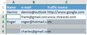
It’s not uncommon to end up with blank cells or rows in an Excel worksheet. If you need to delete these to maintain accuracy, especially when calculating the average value, the quick way is to filter out all blank cells / rows and delete them with one click.
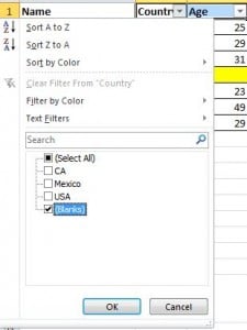
Choose the column you want to filter, go to Data->Filter, after the downward button shows, undo Select All and then pick up the last option, Blanks. All blank cells will show immediately. Now, the blank cells / rows can be deleted easily.
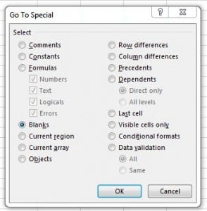
Another way to delete blank rows is to first select blank cells inside the data using the Go To Special feature. It works as follows:
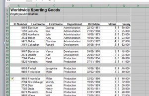
This tool is opened by pressing F5 or by clicking Home, Find & Select, Go to Special. In the Go to Special box, select the Blanks option, then click OK. You will notice that all blank cells in and around the data are now selected.
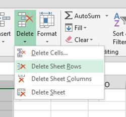
At this point, to delete the empty rows, go to the Home ribbon and click the drop-down of the Delete button in the Cells group. In the drop-down list, click Delete Sheet Rows.
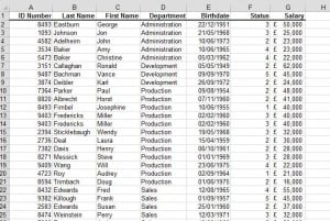
The data will now have no blank rows inside.
Use this method only for simple tables with a couple of dozens of rows that fit within one screen. The main reason is that if a row with important data contains just one blank cell, the entire row will be deleted.
Delete blank rows in Excel using COUNTBLANK
Something we teach on our advanced Excel course: Use this method if you have a table with numerous empty cells scattered across different columns, and you need to delete only those rows that do not have a single cell with data in any column.
In this case we do not have a key column that could help us to determine if the row is empty or not. So we add the helper column to the table:
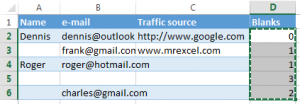
Step 1. Add the “Blanks” column to the end of the table and insert the following formula in first cell of the column: =COUNTBLANK(A2:C2).
This formula, as its name suggests, counts blank cells in the specified range, А2 and C2 are the first and last cell of the current row, respectively.
Step 2. Copy the formula throughout the entire column.
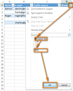
Step 3. Now we have the key column in our table. Apply a filter to the “Blanks” column to show only rows with the max value (3). Number 3 means that all the cells in a certain row are empty.
Step 4. Then select all the filtered rows and remove whole rows .
As a result, the empty row (row 5) is deleted, all the other rows (with and without blank cells) remain in place.
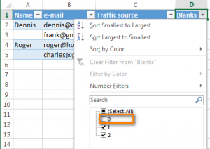
Step 5. Now you can remove the helper column. Or you can apply a new filter to the column to show only those rows that have one or more blank cells.
To do this, uncheck the “0” checkbox and click OK.
