Trying to review a spreadsheet with unformatted data can be a real eye sore, but by using the Total cell style in Excel you can quickly give your data more context.
An example of using the Total cell style in Excel
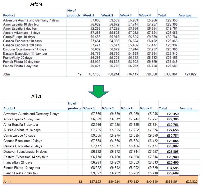
Below we have a list of sales figures for several sales reps in a travel company. In just a few steps by applying the Total style helps the “Total” column of sales figures stand out.

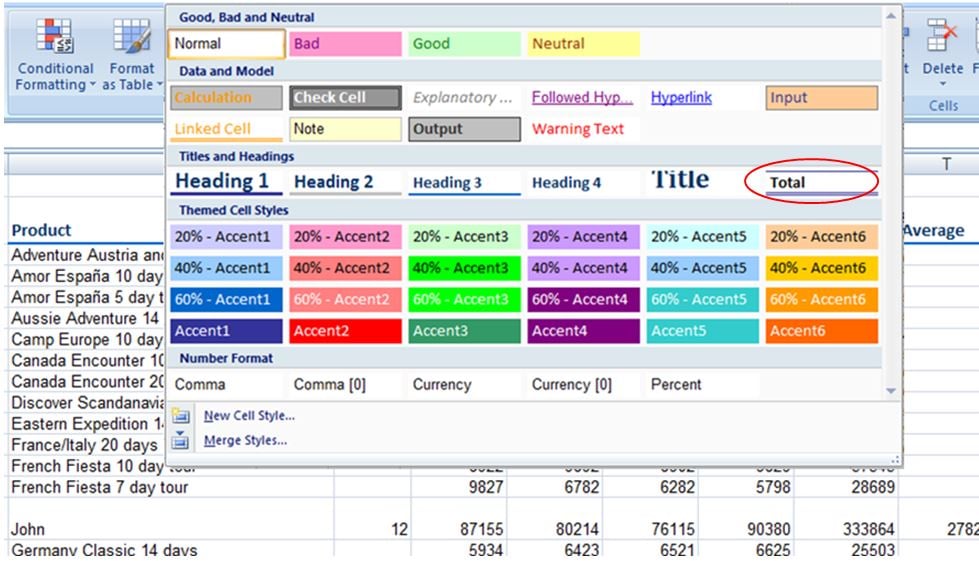
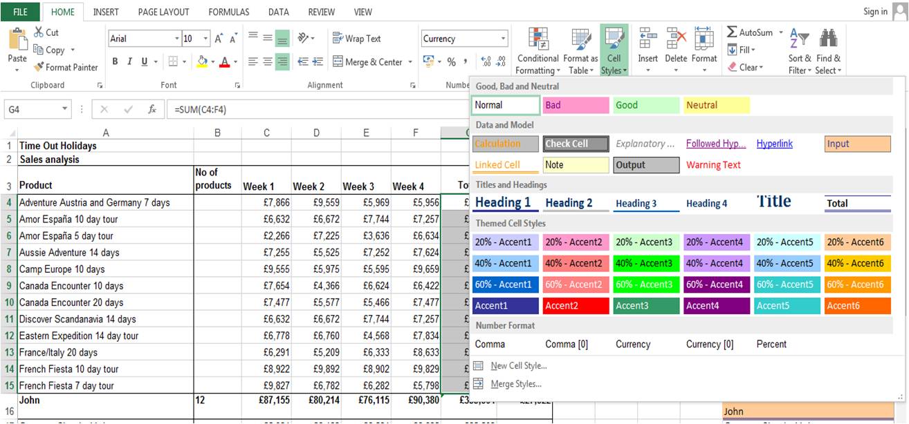
1. Select the range of cells you wish to format. Goto the Home tab, then the Styles group. Then click on the “More” button to expand the group. (for Excel 2013 & 2010 click on Cell Styles button, see the second screenshot below)


2. Now within the Style options, under the section, “Titles and Headings” just select the Total option. The selected range of cells will now display the Total formatting.
In the example above, we also repeated these two steps for the row with “John”, and with one further twist, also included an additional style option under “Themed Cell Styles” which was to select a colour.
Tip: If you are experimenting with different styles you may wish to remove a cell style, to do this simply select the range of cells you wish to “reset”, then go to the Style group (within the Home tab) and select Normal from the “Normal, Bad, Good, Neutral” section.

What we have covered here is a simple demonstration of how using styles can lead to more engaging and professional-looking spreadsheets. You can even create your own custom cell styles which may contain multiple formatting options and can be a real time saver when dealing with similar spreadsheets. We teach this on our more advanced Excel courses London.