An easy to update Gantt chart in Excel
Building a Gantt chart in Excel is pretty easy. But what if you needed to update any of the tasks? This would usually mean lot’s of time consuming manual editing of cells. But there is an easier way….
Step in Excel and the ever flexible conditional formatting function! Yes by deploying some neat conditional formatting tricks you can produce a presentable usable Gantt chart in Excel. You can also learn conditional formatting by attending Microsoft Excel London training course.
Recap: A Gantt chart is made up of task bars, one for each of the tasks required to complete the project in hand. The task bars typically have start and finish dates and therefore have different lengths on duration.
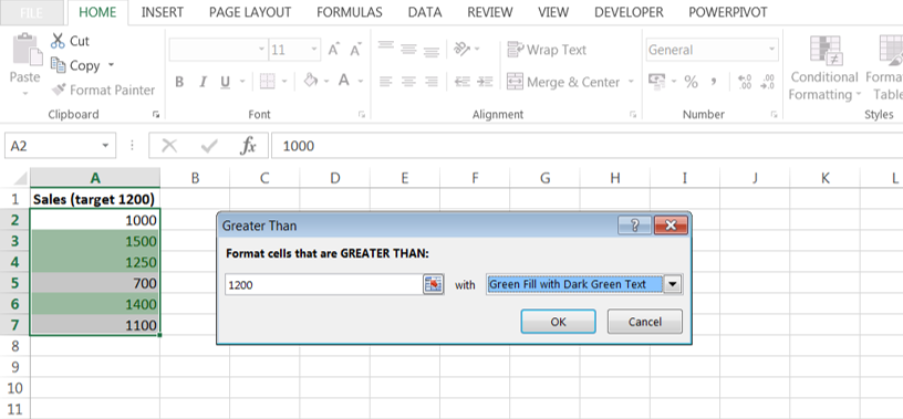
By using Excel’s Conditional Formatting feature we can create our project task bars for our Gantt chart. We will be able to different colour task bars conveniently managed by conditional formatting. An example is shown below on how cell colours can be changed; sales figures green if they exceed a target figure of 1200.
Let’s create a Gantt chart in Excel
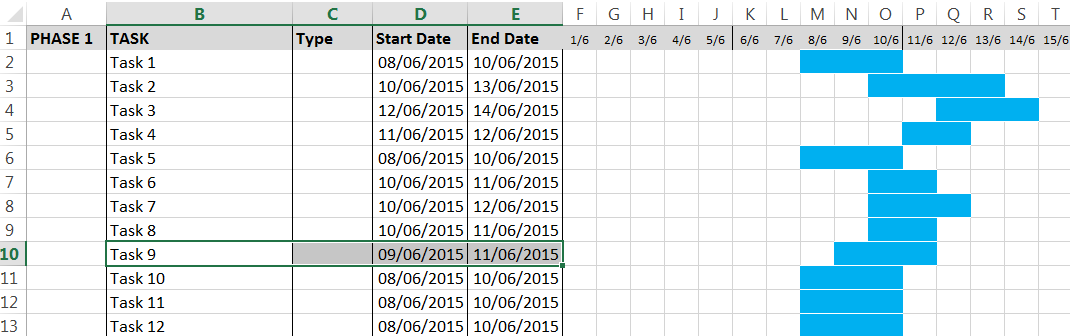
By using conditional formatting we can easily create the following.
Creating the conditional formatting rule
Step 1. Start by selecting the range of cells where bars are to be displayed. In the above example range F2:T11.
Step 2. Select the Home tab then choose Conditional Formatting.
Step 3. Pick New Rule then Choose a formula to determine which cells to format.
In the empty box box (format values if formula is true) enter the formula:
=AND($D2<=F$1,$E2>=F$1)
This formula returns True if a task Start Date is before or equal to the chart date (entered in row 1) AND the Finish Date is after or equal to the chart date.
AND means both conditions within the brackets must apply. The $ sign before a letter means keep that column fixed when applying the rule to the range of cells. Similarly, the $ before a number means fix that row when applying the rule.
Step 4. Now click the Format button and choose a fill colour then OK.
In the example all cells that obey the rule are coloured blue.
Adding more rules
Additional rules can be added for example if certain tasks are designated critical by typing CT in the C column then colour the bars pink.
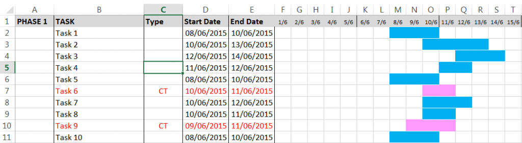
To do this create a new rule as before but include a third condition where the type is CT.
=AND($D2<=F$1,$E2>=F$1,$C2=”CT”)
Click Format and choose pink as the fill colour.
Tips
For consistency you can choose specific fill colour by selecting Fill, More Colours, Custom then entering 255,153,255 for Red, Green and Blue.
Adding a white top and bottom border as part of the Formatting rule can help to separate the bars when touching.
To make changes to colours or to formulas you must highlight the exact range containing the conditional formatting then select Conditional Formatting, Manage Rules. To help do this quickly select Home, Find & Select, Conditional Formatting.
Conditional formats can be copied using the Format Painter.
Additional Resources
Present your data in a Gantt chart in Excel
23 replies on “How to Build an Automatic Gantt Chart in Excel”
would you please send me example of
Additional rules can be added for example if certain tasks are designated critical by typing CT in the C column then colour the bars pink.
Do you have the excel file to download?
Thank you
It won’t work for me at all when I try and include the type column. Can you help?
It won’t work for me at all when I try and include the type column. Can you help?
Thanks! Simple yet very effective excel application. Being looking for similar application since long.
Thanks a ton!!
Your formula does not seem to work for months. Since months have different number of days how is your formula constructed to accommodate that. Thank you.
Great post really helpful. It would be good if you could populate the columns based on a set date without having to create them manually. E.G. If a project started on 1st June, it would populate the dates within say June July and August.
Very cool.
Any option to exclude Saturday, Sunday and public holiday with the formula and color these days in “Grey”?
Hi when I use the formatting =AND(date>=start,date<=end) I am just getting TRUE and FALSE as returns. Please can you expand on fill selection. Many thanks
So I used rule suggested to akin below to get fill, however when I add akin to =AND(E$1=$G14,$E31=”DE”) I not getting second colour fill please can you help what I am missing
=AND(E$16=$G14)
=G16=FALSE
=G16=TRUE
much thanks
I have a weekly time sheet, broken down by 15 minute intervals. Within a given week, I have a multitude of different tasks (manufacturing process steps) that may be applied to different products (items manufactured). In some cases, Task A will begin on Product 1, and at the same time Task G will begin on Product 2. Likewise, Task B may begin at the same time as Task A, on the same Product.
Times are tracked throughout the week for each Task and Product. My goal is to not only color code the different products in each Task row (which your tutorial helps me achieve), but to do so every time said tasks start or stop within the same Task row, and finally to total the time spent performing a given task (regardless of Product).
Is this possible, and can you create a tutorial for this?
Hi guys
Let’s say in addition to formatting/shading the dates I want to allocate 3 people working on a specific project for each day and I want it to pick the number automatically from a specified cell. I want that number to reflect in the cell for each day and end of the month i want to know the total number of staff that worked on different projects on a certain day.
Is that possible?
This was a great help to me. Thank you so much.
YES! Didn’t quite get there the first time – needed to play around a bit – THANK YOU
You need to use both rules, then give the second one a higher priority.
I’m trying to get this formula to work but my dates are in week commencing. therefore what would the formula be to say if the start date is equal to or after the w/c date AND the end date is equal to or after? I’ve tried changing over the in the 1st part but this doesn’t work. I can send the file if that helps – any help much appreciated! Thanks
Great post. Using Google Sheets, but pointed me in the right direction.
I updated to the latest version, and now it keeps on coming up with that tab whenever i startup firefox. What should i do?. I have updated it, there is a tab saying that i have, that is the problem. It is telling me all of the new features that this version offers and everything..
The chart in the example doesnt show dependencies.
I suggest transpose the chart, i.e. make vertical axis as time axis.
It will make the chart much more compact and readable.
Some exmaple in my website.
The formula works great IF there are dates to chart. I have a project plan with planned and actual dates. The actual dates won’t be added until after the task is complete. How do I add to the formula to leave everything blank if there aren’t dates yet? (i.e. IF($G8=””,””)
Once again this post has proved very helpful. Gantt charts are really valuable in giving a quick illustration on how infeeds to a project can delay the entire project.
great information! been google for this formula for the longest time!
i tried both formulas using blank excel sheet , formula ONE is working!!! but formula TWO can’t seem to get it working and i really need this formula.
Seek your help to advise further please?
=AND($D2=F$1,$C2=”CT”)
Can you please send or point me to where I can get this template for downloading?