How to shade alternate rows in Excel – format as table – STL

Here is a quick tip for customising your Excel worksheet.

I like my Excel worksheets to have alternate shading or colours so that it is easier for me to read across rows.

Now, I could set these up manually, by shading in my rows, but if I use sort, or add new rows, the shading will not be alternate. I will get some kind or random stripe effect. What I want is Excel to do, is automatically apply shading to each alternate line, even if I add, or remove a row.

So here is a quick way to set it up

I have a list of students who have all taken an Excel exam.

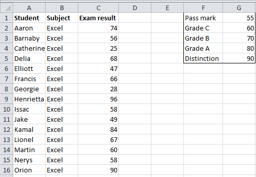
student list plain format excel intermediate training — Here is my list of students. Plain format, so easy for me to read across lines incorrectly.

To make it easier for me to read, I want to add shading on alternate rows.

I select the information I want to shade, including the header, and go to the Home tab, and select Format as Table and select a colour scheme from the options given.

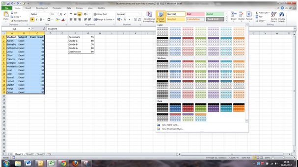
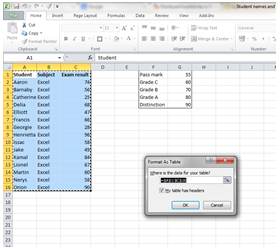
format-table-in-excel-intermediate-training — The Format Table button offers loads of ready made formats to choose from.

I then select the colour scheme I want, and I get a message from Excel confirming the cell range, and whether my list includes headers. My list does, so I click ok.

format-table-message-excel-intermediate-training — Excel prompts me to check that my cell range is correct and to confirm if my selection has a header row.

I can then click out of the selection range and Excel has applied my colour scheme. I can now add student details, or delete rows, and Excel will automatically update the format for me.

I have to admit, I’ve been wanting to be able to do this for ages. One day of intermediate excel training boosted my skills and made it far easier to use the data in my worksheets. If you are feeling curious and want to learn more, take a look at our courses https://www.stl-training.co.uk/excel-2010-intermediate.php.