A new feature introduced in 2010 version of Excel is the Slicer tool. Used to visually and quickly filter data within a Pivot Table.
Although the Pivot Table feature makes it extremely easy to manipulate the layout of data lists in Excel, we have found most attendees of our Excel 2010 training Courses are excited by the power of the new Slicer tool.
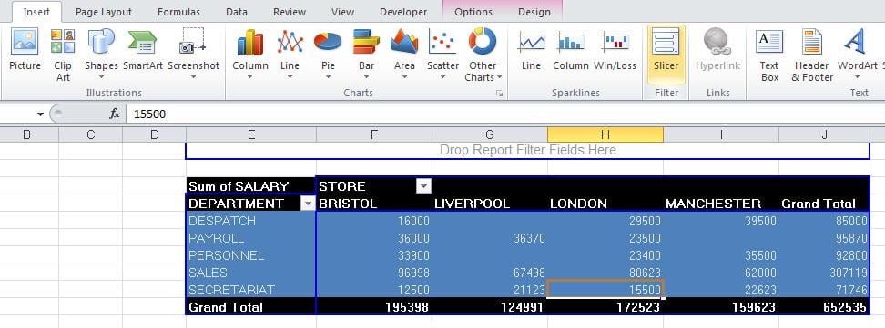
Create a standard Pivot Table and from the Insert Ribbon click the Slicer tool in the Filter Section.
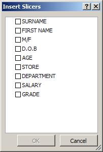
This will display the Insert Slicers Dialog. From the Insert Slicers dialog tick the fields you would like to filter on.
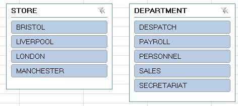
This will display a box for each field selected. These can be moved and resized to suit available space on the sheet.
To filter data, click on the relevant data. In our example below we have chosen the Bristol and London Store with Departments of Sales and Payroll. (You can select multiple items by holding the Control key while clicking).
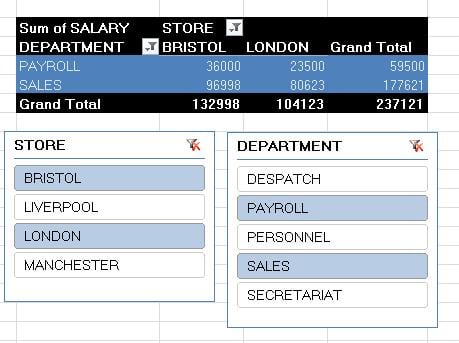
The results are immediate, and the slicer dialogs visually show what is currently filtered.
To clear the filters, click the small funnel icon in the top right of the Slicer boxes.
NOTE: This Slicer feature is disabled if you have workbooks from earlier Excel versions running in compatibility mode. To enable Slicer, Save the workbook as a 2010 file format, then re-open.