How often have you found when you filter Excel data, problems arise in getting it to work? This can happen when you are sharing workbooks or the source data changes frequently. The solution lies in Office 365’s FILTER function. This blog is part 1 of a series that explores the amazing functionality of some of the most popular Office 365 Excel functions starting with the FILTER function.

What is the FILTER function
The FILTER function is based on the standard way of filtering in Excel. It works by extracting the filtered rows from the source data and populating these rows to another sheet. As the filtering process does not affect the source data, we can share workbooks more efficiently. If you have ever struggled using the VLOOKUP to populate specific data into other sheets think again. Why not use the FILTER function instead? It does the same job but, unlike the VLOOKUP, it can return multiple ‘filtered’ rows based on an initial search. Plus, it’s easier to use. So, what’s not to like!
How is the FILTER function different from other functions?
The FILTER function is one of several Office 365 functions that behaves differently to all other Excel functions. With the FILTER function, the results automatically ‘spill’ into all available cells below. In contrast, all other functions require you to copy the result down manually.
How to apply the FILTER function
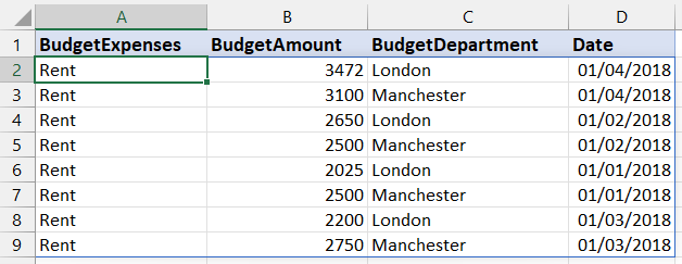
Let’s take some financial data where we will need to filter all records relating to ‘Rent’ (see below)

- Copy the source data headings into another sheet and select the cell below the first heading – see below:
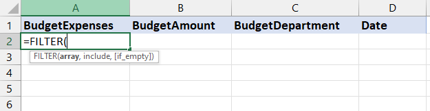

- The 1st part is the ‘ARRAY’ or range of source data to be selected
- The 2nd part is the criteria TO INCUDE in the filter
- The 3rd part (‘IF EMPTY’) is optional and returns an alternate answer if the filter criteria in part 2 does not find a ‘match’ e.g. if there are no records for ‘Rent’ then ‘not found’ is returned in the cell – if this 3rd part was not put in and the criteria was IT equipment, i.e.. not in the list, this would produce an error – see below:

By inserting the 3rd part “not found”, the above error will be converted to this text
As ‘Rent’ is in the list in column A, we get the following filtered results:
One problem that could arise is if there are not enough free rows to populate the results. If any data is ‘blocking’ this space, then you will get a #SPILL error:

To remove the spill error, simply delete the data that is blocking the spill. Other Office 365 functions such as UNIQUE and SORT also have this ‘spill’ feature.
Conclusion
The Excel FILTER function is a great alternative to the VLOOKUP as it is easier to use and can return multiple results based on an initial search. Consequently, the function can help you to improve your efficiency and productivity when you are handling large sets of data.