
Excel isn’t the same spreadsheet program you used a few years ago – Microsoft 365 subscribers get a constant stream of updates that make Excel more powerful and user-friendly. Yet many people haven’t fully explored these enhancements. In our Excel training courses at STL, we often meet experienced users who are surprised by what modern Excel can do.
Below, we highlight five new Excel features (from recent 365 updates) that you might have missed, and why they’re worth knowing. These range from nifty navigation aids to brand-new functions and AI tools. Mastering them can save you time, reduce errors, and supercharge your data work. Let’s dive in!
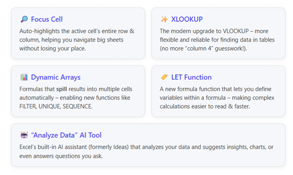
Now, let’s look at each of these features in detail and share a quick tip for using them:
1. Focus Cell – Never Lose Track in Large Spreadsheets
Have you ever scrolled across a giant Excel sheet and lost track of which row or column you were in? Focus Cell is a solution to that problem, introduced in Microsoft 365 Excel in late 2024. When activated, it highlights the active cell’s entire row and column, plus the corresponding headers. The active cell itself gets a thicker border. This makes it super easy to see where you are at a glance – no more squinting or manually shading rows.
- How to Use it: Go to the View tab and click the Focus Cell button (it’s a toggle). Instantly, your current cell’s row and column light up. You can even pick your highlight colour: click the dropdown next to the Focus Cell button and choose “Focus Cell Color” to select a shade that suits you. For example, choose a soft yellow highlight if your sheet has lots of dark colours, so the active row stands out clearly.
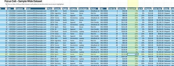
- Why it Helps: In wide datasets or forms, this visual aid prevents entering data in the wrong row by mistake. It’s like having a ruler across your screen – keeping your eyes aligned with the data. Users on our advanced Excel courses love how it reduces errors during data entry or auditing. It’s especially handy if you’re working with frozen panes or split windows, as the highlight stays within each pane to show your position.
- Quick Tip: Use the keyboard shortcut Alt + W + E + F to toggle Focus Cell on and off in Windows. Once it’s on, try using Excel’s Find (Ctrl+F) – each time you jump to a result, that cell’s row & column will be auto-highlighted (Excel auto-activates Focus Cell during Find & Replace by default). This makes scanning search hits much faster in large sheets. And if you love it, add the Focus Cell toggle to your Quick Access Toolbar for one-click access.
Bottom line: Focus Cell is a small tweak that yields a big productivity boost. If you frequently work on big spreadsheets, turning this on can feel like putting highlighter tape on your screen – simple but game-changing for your focus.
2. XLOOKUP – The Better VLOOKUP
For decades, VLOOKUP was the go-to function to search for a value in a table. But it had notorious limitations: you had to count column index numbers, it couldn’t look left, and it defaulted to approximate matches which caused errors. Enter XLOOKUP – a newer lookup function available only in Excel 365 that fixes virtually all those issues.
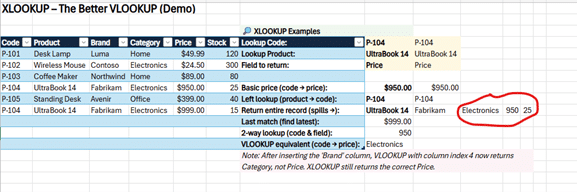
What it Does: XLOOKUP finds things in a table by column or row, in one function. For example, with XLOOKUP you can search for a product code in column A and return the price from column F without needing those columns to be in any specific order. It’s as simple as:
=XLOOKUP( lookup_value, lookup_array, return_array, “Not found”)
No more cryptic “column_index_num” – you specify the exact ranges. It can look to the left (VLOOKUP couldn’t), and by default it looks for exact matches (reducing errors). It also can return a whole row or column of results (when combined with dynamic arrays – more on that soon). In short, it’s a one-stop replacement for VLOOKUP, HLOOKUP, and even a lot of INDEX/MATCH uses.
- Why it’s Useful: Fewer headaches and mistakes! If you’ve ever had a VLOOKUP break because someone inserted a new column, or you got the dreaded #N/A due to the function not finding an approximate match, XLOOKUP is a relief. It’s more intuitive: you tell Excel “here’s what to find” and “here’s where to look” and “here’s the result to give me” – that’s it. For example, on our courses we show how an XLOOKUP can fetch a customer’s entire record in one go, whereas VLOOKUP would need multiple formulas.
Also, XLOOKUP can search from bottom up (useful for finding the last occurrence of something) and can perform 2-way lookups (find value at intersection of a given row and column) with a single formula.
Quick Tip: Replace your old VLOOKUPs with XLOOKUP when you can. The syntax is straightforward:
XLOOKUP(value, lookup_range, return_range, [if_not_found], [match_mode], [search_mode])
The handy [if_not_found] argument lets you return a custom message like “Not in list” instead of an #N/A error if the value isn’t found. This makes your spreadsheets more user-friendly. Also, remember XLOOKUP isn’t available in Excel 2016 or 2019 – it’s a Microsoft 365 feature.
So if you share your file with colleagues on older versions, consider that (or suggest they upgrade!).
But if you have Excel 365, embrace XLOOKUP; it will simplify your lookup formulas greatly. In our Excel Advanced training, learning XLOOKUP is often an “aha” moment for folks who have wrestled with VLOOKUP’s quirks for years.
3. Dynamic Arrays – Formulas That Spill (FILTER, UNIQUE, SEQUENCE and More)
This one’s a bit more advanced, but massively powerful: Dynamic Arrays. Traditional Excel formulas return a single value per cell. Dynamic array formulas, introduced around 2020 for Office 365, can return multiple results that spill into adjacent cells automatically. Microsoft also introduced a suite of new functions to leverage this: notable ones include FILTER, UNIQUE, SORT, SEQUENCE, and more. If you haven’t heard of these, you’re in for a treat.
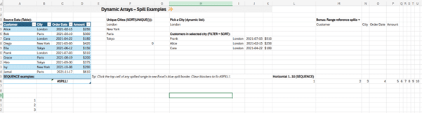
- What it Means: With dynamic arrays, you can, for example, write one formula to extract all customers from London from a data table, and Excel will spill the list of names into as many cells as needed. The formula might be:=FILTER(Table1[Customer], Table1[City]=”London”)If 25 customers match, you’ll see 25 results populate downward automatically. If you then change the city to “Paris”, the array resizes. No need to copy formulas down or worry about ranges – Excel adjusts the output dynamically.
The new UNIQUE function works similarly:
=UNIQUE(range) will output a de-duplicated list of all unique values from the range. SEQUENCE can generate a list of numbers (e.g., 1 to 100) across cells with one formula. These are tasks that previously required manual work or complex tricks. Dynamic arrays have essentially changed how formulas work under the hood, allowing this fluid spilling behavior.
- Why it’s Useful: It simplifies complex tasks. Consider making a summary table of data that meets certain criteria – before, you might use pivot tables or complicated array formulas with Ctrl+Shift+Enter. Now, a single FILTER or UNIQUE formula can do it intuitively. It’s also volatile in a good way: when your source data changes, the results update live. If your unique list grows, Excel will automatically extend into empty cells below; if it shrinks, it clears the now-unneeded cells.This dynamic nature turns Excel into more of a responsive canvas. Our trainers often demonstrate dynamic arrays by showing how to build interactive drop-downs: you can point Data Validation to a dynamic array range, so the list of options updates itself based on data – no manual range resizing.Beyond new functions, even traditional functions can spill: try typing =A1:A5 in a cell and pressing Enter in Excel 365 – you’ll see it spills the 5 cells’ values horizontally (a nifty surprise!).
- Quick Tip: If you experiment with a dynamic array formula and see #SPILL! error, it means something is blocking the cells where the results want to spill. Simply clear any data below/next to that cell, and the array will flow out.To visually grasp dynamic arrays, use the new “spill range” highlighting: when you click the top cell of a spilled range, Excel puts a blue border around the entire range of results. And if you click any other cell in that range, the formula in the formula bar appears ghosted (because the actual formula lives in the first cell).This is Excel’s way of saying “these cells are outputs of a single formula”. One more tip: dynamic array functions are available on Excel for web and mobile too – so your spreadsheets with these will work consistently across devices.
In short: dynamic arrays let Excel do more heavy lifting for you. They’re a bit advanced, but we include an introduction to functions like FILTER and UNIQUE in our Excel Advanced courses now, because they enable elegant solutions that were impossible or very tedious with older Excel. If you love efficiency, they’re worth learning.
FILTER Function Example
Using Excel’s new =FILTER function, you can produce a permanent dynamic filtered result from a data set. First, you need to convert your data set to a Formatted Table:
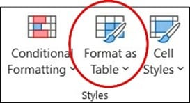
This is found in Excel’s Home ribbon.
Here is an example of an =FILTER result from a formatted table:
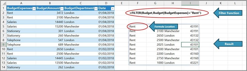
The data set has been renamed as ‘Budget’. Because the data set dynamically grows with new entries, the =FILTER result will automatically update and show any new rows which match the filter criteria. The =FILTER Function is a Spill type function, which means you type it into one cell and it automatically ‘spills’ into more cells to show the result.
4. LET Function – Simplify (and Speed Up) Complex Formulas
If you’ve ever written a mega-formula in Excel, you know it can get hard to read and maintain. The LET function (new in Microsoft 365) is here to help with that. It allows you to assign names to sub-expressions within a formula, similar to how you might use variables in programming. This makes formulas easier to understand and can improve performance by avoiding repetitive calculations.
- How LET Works: The syntax is LET(name1, value1, name2, value2, …, calculation_using_those_names). You define one or more names and their corresponding values, then specify a final expression that can use those names.For example:
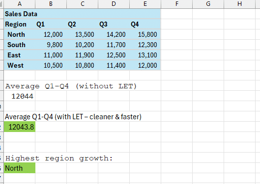
=LET(total, SUM(A1:A100), count, COUNTA(A1:A100), total / count)This computes the SUM and the COUNT once each, names them, and then the last part total / count gives the average. In a normal formula, you might write SUM(A1:A100)/COUNTA(A1:A100).That works, but it calculates the sum and count separately. With LET, you calculated each only once, then reused the results. For large ranges, that can speed things up. More importantly, if you look at the LET version, it’s clearer what’s happening: you see “total” and “count” which are meaningful, rather than repeating A1:A100 and having to mentally parse it.

- Why it’s Useful: Clarity and efficiency. It’s like giving your formula some breathing room by breaking it into parts. When you or a colleague come back to that formula later, those intermediate names make it far more readable.
Performance-wise, Microsoft noted that LET can make big worksheet models faster because it reduces duplicate calculations.Imagine a complex nested IF or a heavy array formula; using LET to calculate a sub-term once (like a complex criteria or a long reference) and reuse it means Excel does less work. For example, if you have an index formula that uses the same SEARCH() calculation twice, wrapping it in LET to do SEARCH once and store it can cut calculation time roughly in half (this is a common trick in financial models now).Another real scenario: we helped a client rewrite a monstrous formula for commission calculations using LET – it went from an unreadable 4-line formula to a cleaner one with named steps like basePay, bonusRate, etc., and it recalculated noticeably faster across thousands of rows. - Quick Tip: Don’t be intimidated by the syntax. Start by using LET in formulas where you notice repetition. A good pattern is to use it to avoid writing the same VLOOKUP/XLOOKUP or calculation twice.For instance:
=LET(x, XLOOKUP($A2, ClientIDs, PlanType), IF(x=”Premium”, 0.1, 0.05) * Revenue)Here we XLOOKUP the client’s plan type once, name it x, then use x twice in the IF. Without LET, you might have had to either do two XLOOKUPs or pull that value into a helper column. LET saves you from that.
Remember that names in LET are only valid inside that formula – they don’t conflict with named ranges or anything globally. Also, you can nest LETs inside each other if needed (though that might get a bit hard to follow).In summary, use LET to tame your monster formulas; your future self will thank you. It’s a great example of Excel adopting programming concepts to make advanced users’ lives easier.
5. “Analyze Data” – Excel’s AI Helper for Insights
Excel isn’t just about manual formulas anymore – it also has built-in AI to assist you. The feature Analyze Data (formerly known as “Ideas”) lives in the Home tab and leverages Microsoft’s AI to analyze your dataset and suggest insights, trends, and even generate visualizations or formulas. It’s like having a little data analyst inside Excel.
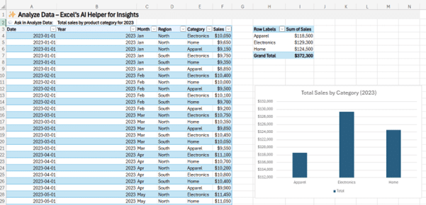
- What it Does: When you click the Analyze Data button, Excel looks at the data in your worksheet and comes up with useful nuggets: summaries, outliers, patterns. For example, it might tell you “July had the highest sales overall” or “Region South is an outlier in Q4”.It often suggests charts or PivotTables – and you can insert those with one click if you like the insight. What’s more, there’s a Q&A box where you can type a question in plain English (or other supported languages) about your data.For instance, you could ask: “Total sales by product category for 2023” – the AI will generate a PivotTable or chart answering that if it can interpret the data. It uses natural language processing, so you don’t have to write a formula or code; you just ask, and Excel will try to figure it out.
Think of it as an AI-powered analyst that can do some of the thinking for you, within limits. - Why it’s Useful: Not everyone is an Excel guru, and sometimes you don’t even know what you’re looking for in a big dataset. Analyze Data can quickly point you to interesting insights or at least give you a starting point.It’s great for sanity-checking your data: if the AI highlights a trend (“sales have been increasing month-over-month”) that you weren’t aware of, that’s valuable.
Or if you’re not fluent in PivotTables, the fact that it can generate one for your question is a big time-saver. Even advanced users appreciate it for rapid exploration – it’s like getting a second pair of eyes on the data.From a training perspective, we find that showing newcomers the Analyse Data feature early on helps demystify data analysis; they see that Excel can do some heavy lifting. It’s also a glimpse of where Excel has been heading with AI.Today, that vision is here: Microsoft Copilot is now fully integrated into Excel, making it easier than ever to work with data. You can simply ask Excel in natural language to build formulas, create dashboards, summarise trends, or even generate insights – all without needing to know complex syntax.And if you’re curious about what’s next, check out Excel Labs. It’s an experimental space where Microsoft tests innovative features before they go mainstream. Excel Labs gives you early access to cutting-edge tools and ideas, so you can explore what’s coming and help shape the future of Excel.Copilot and Excel Labs together make Excel not just a spreadsheet tool, but a smart, evolving platform for data analysis and decision-making. It’s no longer just on the horizon – it’s here, and it’s transforming how we work with data.
- Quick Tip: To use Analyze Data, put your data in a proper table (Insert > Table) or at least have it well-organized with headers – the AI works best when it can clearly identify your dataset’s structure.
Click anywhere in the data and hit Analyze Data on the Home ribbon. If you have a specific question, type it where it says “Ask a question about your data”.For example, type “average score by category” or “total expenses by month as line chart” – be relatively concise and use your column names in the question for best results.If Excel can’t figure it out, try rephrasing (it’s a bit like talking to a search engine). Also note, if your data range is too large or complex, Excel might say it can’t analyse (there are some limitations – e.g. it usually won’t work on over a million cells, or if your workbook is very messy).Start with a clean dataset. And remember, any charts or summaries it creates are inserted into your workbook so you can tweak them further. It’s not perfect – think of it as a helpful assistant that might not catch everything, but often produces useful results.Many of our Excel training attendees are surprised to see Excel can do this – it’s a hint that learning Excel now isn’t just about manual formulas, but also about leveraging AI tools to work smarter.
Wrap-Up: These five features – Focus Cell, XLOOKUP, Dynamic Arrays, LET, and Analyze Data – showcase how Excel (especially the Microsoft 365 version) is evolving.
If you hadn’t heard of some of them, it’s a great time to explore. They can make everyday tasks easier and open up new possibilities in what you can do with Excel.
The best part is that our Excel courses at STL are continually updated to include these new capabilities. We don’t just teach you Excel as it was – we teach it as it is now.
That means when you attend, say, an Advanced Excel training, you’ll learn about XLOOKUP and FILTER, not just VLOOKUP and AutoFilter.
We ensure you walk away with knowledge that’s relevant to the current version of Excel, so you’re not missing out on tools that could save you hours.
Excel is a bit like a Swiss army knife that keeps getting new attachments. It’s worth keeping up with what’s new, because you might find a feature that addresses a pain point you’ve had for years.
Hopefully, at least one of the tips above made you go “I didn’t know Excel could do that!” – in which case, go try it out. And if you want a deeper dive into mastering these and many other Excel tricks, you know where to find us (shameless plug: our Excel training workshops face to face or online will get you hands-on with all this good stuff).
Happy Excelling – may your spreadsheets be ever efficient!