Easily copy & paste using the Transpose option
This is a very useful little tool (and one of many that we cover on our Advanced Microsoft Excel courses). Sometimes when setting up a worksheet you may realise that it would be better to put your column data into a row. One way to achieve this would be by cutting and pasting individual cells. But there is a more efficient way.
There are lots of pasting options – here is a quick example of how the Transpose option works.
To change vertical data in a column to horizontal data in a row:
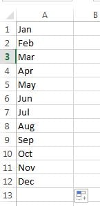
Step 1. Copy the vertical data. In this case months of the year can be used as a simple example. Just click and drag to select the text, and then Control + C to copy it.
Step 2. Find the cell you want to insert the data, and then click on it to select.
Step 3. Select the Paste button, but click on the down arrow – and a pop up menu of choices appears (these are your Paste Special options).
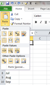
Step 4. Select the Transpose option and click ok…and your vertical data is now across the top row

Tip: You can also access the Transpose option, by right clicking when you have selected the new destination cell, and you can select Transpose icon from the Paste Special menu.
You can use the Transpose option to paste Horizontal data to the Vertical using the same method.
It’s a really simple tool that can save significant time and allow you to develop your worksheets without having to redesign everything if you decide to switch rows, to columns. Other paste options are included in our advanced Microsoft Excel courses https://www.stl-training.co.uk/excel-2010-advanced.php.